What is blooming in night-light satellite data?
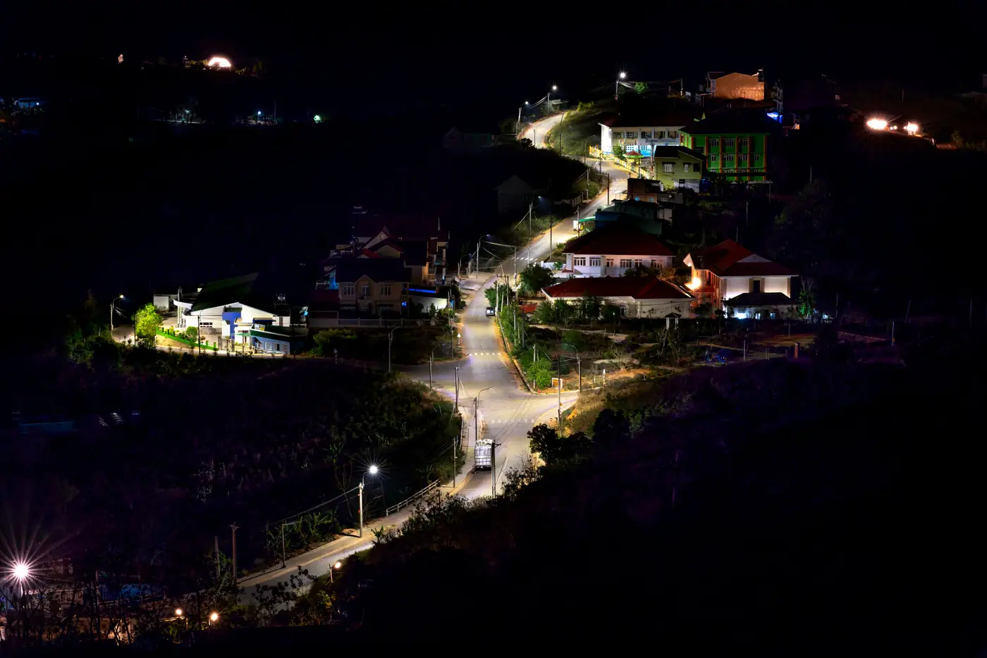
If you've pulled a VIIRS night-light tile over one of your financed sites and compared it to the feeder route on the engineering drawings, you've probably noticed the lit patch spills well past where the transformers and poles sit. That spill has a name: blooming. It's a sensor artifact, not a sign that the grid reached further than the drawings say.
Why a light source looks bigger than it is
Night-light sensors like the VIIRS Day/Night Band don't photograph settlements the way a camera photographs a building. They record radiance at a ground resolution that's coarse by design, commonly in the 500-750 m range for VIIRS, because the instrument is built to catch faint light at night across the whole planet, not to resolve individual streets. A single bright point, a transformer yard, a market strip with new floodlights, a cluster of connected households, saturates the pixel it sits in and then leaks brightness into the pixels around it. Add atmospheric scatter and the sensor's own optical blur, and a 200-meter cluster of newly connected homes can show up as a glowing patch several times that size on the map.
Most people tracking electrification between surveys use night-light data as a stand-in for census or utility figures, drawing a boundary around where the lights are visible and calling that the settlement's footprint. Blooming inflates that boundary. A programme area that looks like it has 40 hectares of lit territory might have a tenth of that actually wired. That gap comes from the optics of the sensor, not from fraud or bad data entry at the utility.
Blooming is uneven, too. A single large, very bright point source, say an industrial facility or a well-lit highway interchange, blooms more than several smaller sources spread across the same area, even if total connected load is similar. Comparing the apparent size of two settlements' light patches year over year tells you less than you'd hope about which one added more connections, because the brighter source will always look disproportionately large.
What you can still read from the data
The fix is to change what you're measuring. Instead of asking how big the lit area is, ask how brightness at a known point has changed since last month. Hold your sample points fixed, the settlement centroids, substation locations, the village markets you already surveyed, and blooming affects each one in roughly the same way each month. The artifact becomes a constant you can mostly ignore, and the month-to-month change in intensity at that fixed point becomes a reasonable proxy for whether more load came online nearby.
That's a different discipline than most people bring to a night-light tile the first time they open one. Track a time series at defined coordinates: compare this month's read to last month's for the same point, rather than comparing the apparent size of two different lit patches to each other.
It also means not expecting pixel-level precision. At a resolution of 250 meters or coarser, you're not going to see which specific household got connected. You're seeing whether a settlement, as a unit, is getting brighter or staying flat, which is a more honest question than how far the grid extended.
For a portfolio economist checking on financed projects between formal survey rounds, that's often enough. A monthly intensity read across your programme area won't replace the household survey due at midterm, but it gives you a signal of whether things are moving in the gap years when the survey isn't due. Electrification Map builds that monthly read as a single panchromatic layer over the settlements you're tracking, so you can watch intensity trend at each site instead of trying to eyeball a bloomed boundary.
If blooming has been making your footprint estimates look better, or worse, than reality, it's worth switching to a point-based monthly read instead.